OpenStreetMap (OSM) is an open, community-maintained base map of the world. It includes the outlines of countries, locations of cities, important places and landmarks, natural features like rivers, and roads – all of which can be important for businesses looking to perform geospatial analytics. Especially when customers must travel to a retail store front, the distance from a major road and proximity of other places plays a major factor and OSM data can help provide those key insights.

In Hex Tiles, an analytic data tiling system that Foursquare launched just this past year, data is projected into a hexagonal H3 grid system in order to have a common unit for joins. The uniform grid of hexagons provides a convenient way to define analytics on top of the joined data. Our previous post expands more on why transforming data from its source geometry into the H3 grid is useful.

The data source

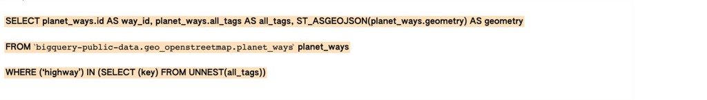
We used the BigQuery OSM dataset to export features. This allows us to query for features of interest, such as highways (which, in OSM terminology, refers to any motorway or pedestrian path), railroads, or buildings.

These offer an easier way to query OSM than downloading and processing snapshot files. As an example, a query would look something like:

Selecting highways in OSM is a little different than one might think. In OSM, the term highway refers to “any road (…) on land which connects one location to another and has been paved or otherwise improved to allow travel by some conveyance, including motorized vehicles, cyclists, pedestrians (…) but not trains.” Highways under this definition also include pedestrian and bicycle paths that are not traversable by cars at all. This is quite extensive compared to the American English definitio: “a main road, especially one between towns or cities.”

OSM uses tag values and other tags to differentiate between types of ways. For example, a pedestrian way might be tagged as highway=path or highway=footway, a local street as highway=residential, and a major freeway as highway=motorway.

The OSM definition of highway excludes all trains and railways, so trams, metro lines, and rail lines must be queried separately. The query and processing for railways are very similar to that of highways, besides replacing the tag key with “railway.”

Projecting roads

Once we have all the OSM features of interest, we want to project these vector geometries into the H3 grid. For linestring geometries like roads and railroads, we can do this by using the h3Line library function, or by interpolation of points using another geometry library, Shapely.

In addition to marking that a road is present in a cell, we can calculate the sum of road feature length in each cell.

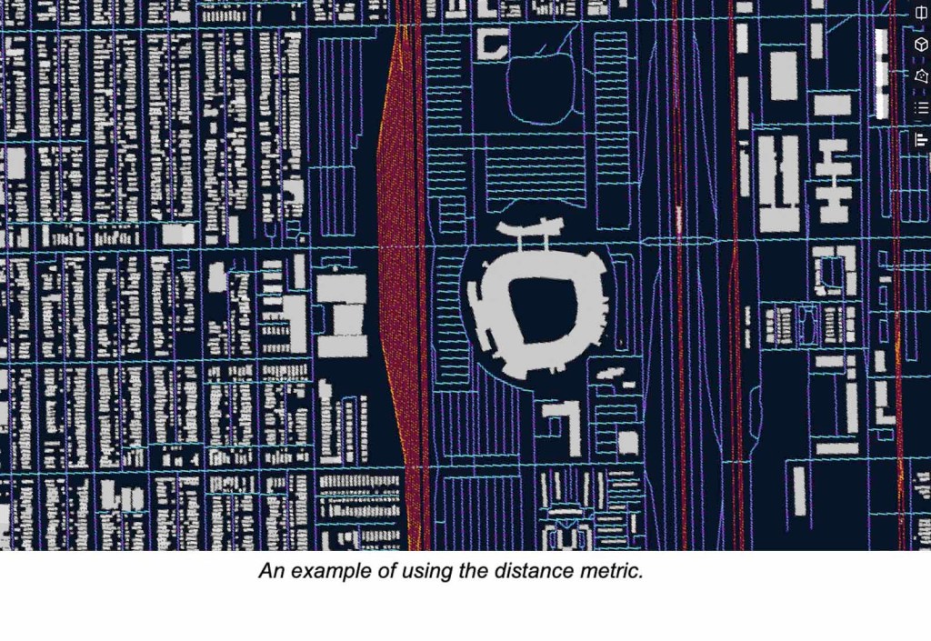
Coverage of roads can be used in lieu of a basemap and is enough to visualize the basics of the street network. When transferred into a Hex Tile format, it can be immediately brought into H3-based analytics to help answer additional questions such as is this point on a road segment, how far is this point from the nearest road segment, and more.

Certain parts of rail lines show higher distance value, the reason being there are multiple rails at those areas such as rail switches.

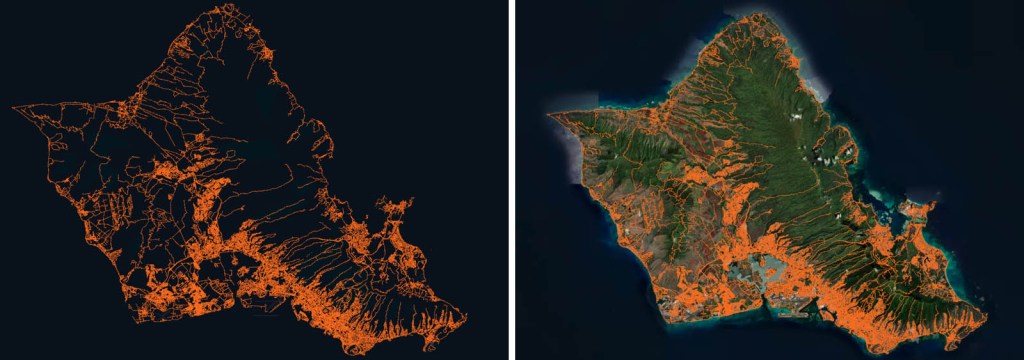
We can also zoom out our Hex Tiles to get a broader view of the OSM dataset. This is particularly useful for checking the coverage of a geospatial dataset.

Comparison with TIGER

OSM includes some Topologically Integrated Geographic Encoding and Referencing (TIGER) data, which is a public domain data source produced by the United States Census Bureau. This dataset is also available in Unfolded Studio’s data catalog as Hex Tiles.

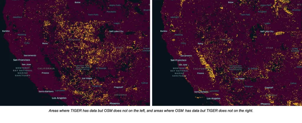
Hex Tiles are designed for analytical joins. Comparative analysis from joining the OSM and TIGER datasets tells us how coverage differs for these two datasets. When joined, it is simple to define metrics as OSM data is present and TIGER data is not present because both TIGER and OSM columns are available on each row of data. When either TIGER or OSM data is not present in that area, the values in those columns will be null.

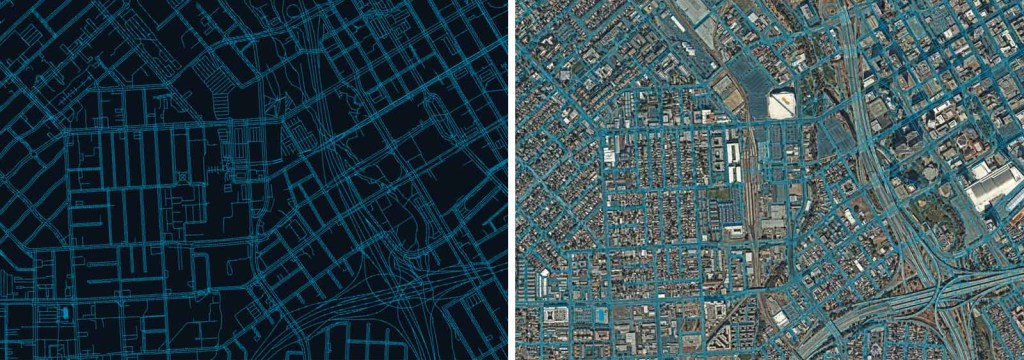
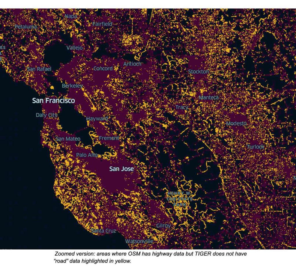
In the figures above, joins are used to evaluate the coverage of the two datasets. One does not stand out as a superset of another when zoomed out. However, when zooming in, the data reveals that OSM tends to have more complete coverage of individual roads and paths. In our experience, the OSM dataset is the more comprehensive and precise of the two.

Above we can see some micro-differences in the OSM and TIGER datasets. In these examples, TIGER (left, orange) data is missing segments and is of lower precision than OSM (right, blue) data. Clearly Caltrain, an operating railroad, should have rails that connect!

Projecting buildings

The OSM dataset contains building polygons which we can project into Hex Tiles as well.

Building polygons project into H3 is slightly different than they do for roads. For building polygons, we chose to use the H3 library’s polyfill function, combined with projecting very small buildings as a single point. This allowed us to correctly mark all areas that OSM has building coverage.

Similarly to roads, we also include the sum of the area of buildings within a cell when multiple buildings overlap or when buildings have outlines with more detail than the H3 cells we use to represent them.

Hex Tiles carry aggregate data, not data for individual buildings. Still, it’s very useful to include OSM feature IDs and building information in our Hex Tiles since this represents the building at that particular location for non-overlapping buildings. We can choose how to resolve which OSM feature ID to include in Hex Tiles in a few ways. One is to choose a simple aggregation function like min or max. Another is to choose based on some aspect of the buildings, such as the height or area, so that the taller or larger building is chosen.

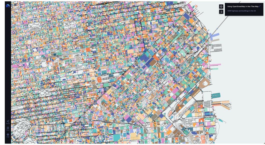
Hex Tiles give us an immediate sense of the coverage of these datasets. Above we see OSM coverage of buildings in the northeast United States. We can clearly see artificial lines where data has been imported from some areas but with much spottier coverage across those boundaries. This likely reflects specific counties or cities where more work has gone into cataloging buildings in OSM.

Join with heights

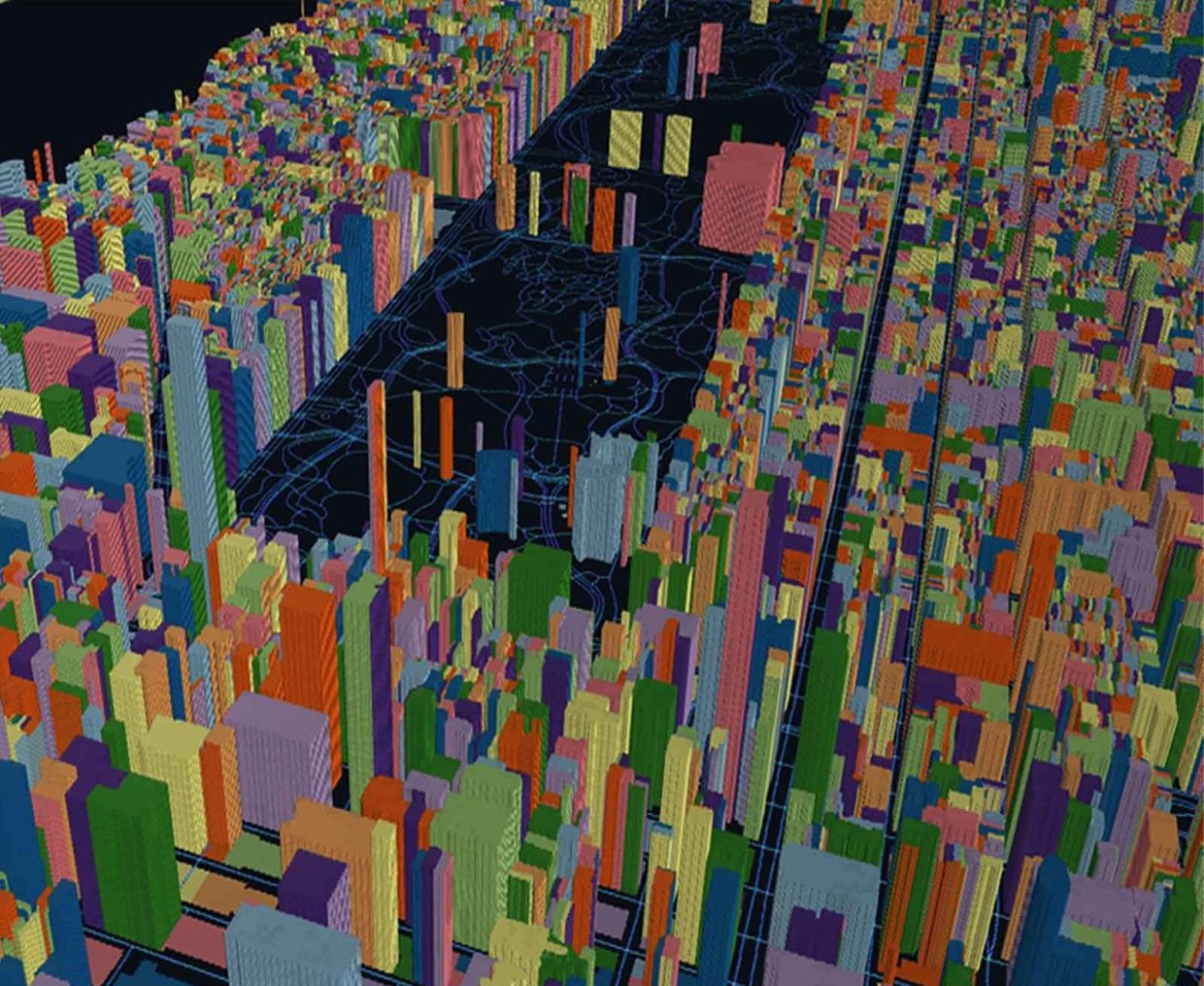
Combining the roads, railroads, and buildings into a single, three dimensional map visualization lets us build a sort of hex-based digital twin in Unfolded Studio. OSM provides the heights of some buildings in an optional height tag. We can use the height of the buildings to extrude them and show their 3D nature in comparison to the roads around them.

The OSM datasets mentioned above are now available in the Unfolded Studio Data Catalog under Infrastructure. We currently have US highways, US buildings, and global railroads available, and encourage you to explore the platform and develop your own maps.

All the OSM data in this blog post is copyrighted by OpenStreetMap contributors and available for free under the ODbL license.