Segmentation is a crucial aspect of modern marketing, allowing companies to divide their audience into meaningful groups based on common characteristics, behaviors, and preferences. By incorporating segmentation into planning, marketers can better understand and tailor their messaging to specific audiences, leading to more personalized and effective campaigns.
One of the simplest and most popular methods for creating audience segments is through K-means clustering, which uses a simple algorithm to group consumers based on their similarities in areas such as actions, demographics, attitudes, etc. This mini-tutorial will demonstrate how to get started with K-means clustering in Python using the scikit-learn library and ways to create audience segments that can inform marketing strategies.
Introduction to K-Means Clustering
K-means clustering is a widely-used unsupervised machine learning technique for data segmentation. It aims to partition a set of points into K number of clusters based on their similarity, such that the points in a cluster are as close to each other as possible and as far from the points in other clusters as possible. The algorithm iteratively updates the centroid of each cluster, which is the average of all points in the cluster, until the centroids no longer change or a maximum number of iterations is reached. The final result of the K-means algorithm is a set of K clusters, each with a designated centroid, that best represents the structure of the data.
In order to use K-means clustering to segment an audience, it is important to first consider what aspects you would like to use to segment the consumers. These aspects could be demographic information, behaviors, attitudes, etc. Once the aspects have been determined, a DataFrame profiling each consumer on each aspect can be created.
In the following sections, we will show you how to prepare the data for K-means clustering, including standardizing the features and reducing the dimensionality through use of Principal Component Analysis (PCA). By the end of this tutorial, you will be able to use scikit-learn in Python to create meaningful audience segments using K-means clustering.
Importing Required Libraries in Python
We will utilize pandas and NumPy to work with our data; scikit-learn to perform dimensionality reduction and K-means clustering; then Matplotlib and seaborn to visualize the results.
import pandas as pd
import numpy as np
from matplotlib import pyplot as plt
from mpl_toolkits import mplot3d
import seaborn as sns
from sklearn.preprocessing import StandardScaler
from sklearn.decomposition import PCA
from sklearn.cluster import KMeans
from sklearn.metrics import silhouette_samples, silhouette_score
Preprocessing and Feature Engineering the Data
Before we dive into the technical aspects of clustering, it’s important to first identify the key characteristics that will be used to segment the consumers. In this tutorial, we will work with a data set of users on Foursquare’s U.S. mobile location panel, aiming to uncover unique holiday shopping segments in order to describe their behaviors and enable advertisers to reach them.
We looked at users’ holiday season retail visitation behaviors that were most important to our clients, including types of stores visited; visits per user (VPU) per active day; distance traveled; dwell time; and temporal aspects. We also included demographic aspects such as predicted age and gender, income, and population density.
This information is compiled into a pandas DataFrame, with rows being individual users, and columns being the features we defined above. The visual below shows a sample of the ~100K users and 16 features in our DataFrame:
df.head()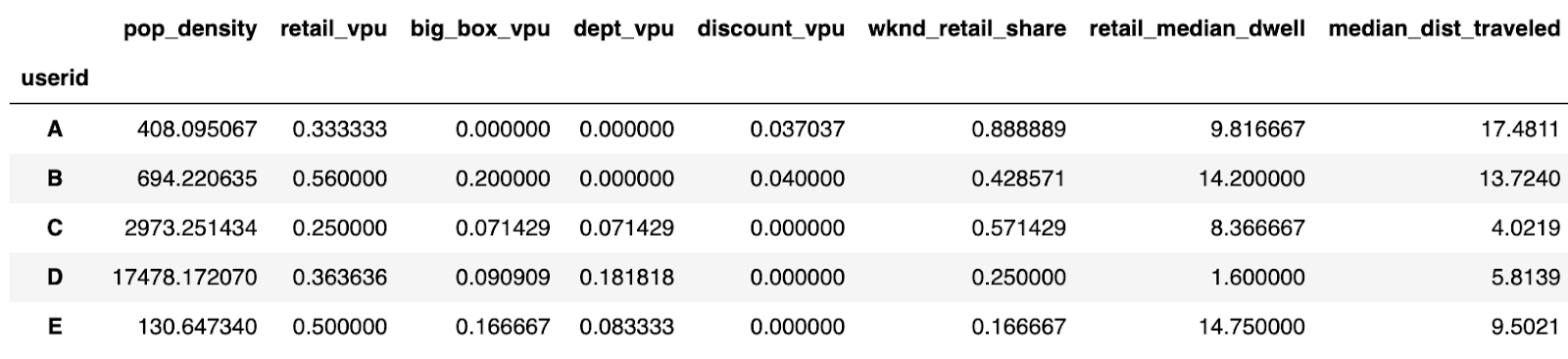
Before we can proceed with the next step, it’s important to standardize our features. This is crucial because the dimensionality reduction and clustering algorithms we will use in this tutorial are not scale-invariant. In other words, the results of these methods can be greatly influenced by the units and scales of the features in the data set. By standardizing the features, we ensure that each feature contributes equally to the analysis, leading to more accurate and meaningful results.
There are multiple ways to standardize the featureset, but in this case we found the best results when bucketing each feature into quantiles using the pandas qcut function, then using sklearn’s StandardScaler preprocessor. StandardScaler works by removing the mean and scaling to unit variance so that each feature has μ = 0 and σ = 1.
# Define which columns contain our features
feature_cols = df.columns.to_list()

# Discretize each column into quantiles
for column in feature_cols:
  df[column] =
pd.qcut(df[column].sort_values().rank(method='first'), q=5,
	duplicates='raise', labels=False)

# Convert to a numpy array
X = df[feature_cols]
X = np.array(X)

# Scale the values
scaler = StandardScaler()
scaler.fit(X)
X_scaled = scaler.transform(X)
X_scaled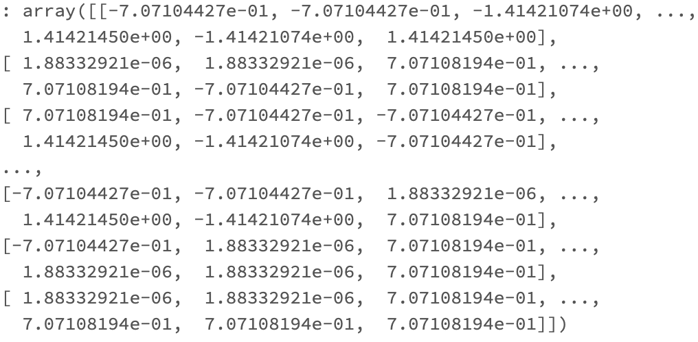
Dimensionality Reduction with PCA
Principal Component Analysis (PCA) is a commonly used method for dimensionality reduction and provides significant benefits for clustering analysis. Our data set has 16 features and is therefore 16-dimensional, which is not ideal for performing K-means clustering. The more features we have, the more likely we are to encounter the “curse of dimensionality” when we attempt K-means clustering. This is a phenomenon in which the distance between data points in high-dimensional space loses meaning, making it difficult to accurately cluster the data.
By reducing the number of features using PCA, we can mitigate the curse of dimensionality impact and improve the accuracy and efficiency of our K-means clustering analysis. PCA works by transforming the data into a new coordinate system where the first few axes, or principal components, capture the most variance in the data This allows us to capture the most important patterns and relationships, while simplifying the analysis.
We first need to determine how many principal components to move forward with. We can do this by looking at the cumulative explained variance for each principal component and choosing a number of principal components that captures a sufficient amount of the variation in the data, while still reducing the dimensionality.
# Instantiate PCA
pca = PCA(n_components=16, random_state=99).fit(X_scaled)

# Store explained variance results in a DataFrame
evar_df =  pd.DataFrame(data=pca.explained_variance_ratio_,
		index=range(1,len(feature_cols)+1))
		.rename(columns={0:'pct_explained_variance'})

# Calculate cumulative explained variance
evar_df['cum_explained_variance'] = evar_df.cumsum()

# Plot using matplotlib
fig = plt.figure(figsize=(6,4))
ax = fig.gca()

sns.lineplot(data=evar_df, x=evar_df.index,
		y='cum_explained_variance', ax=ax, color='blue')
		.set_title('PCA Cumulative Explained Variance')
plt.ylabel('cumulative explained variance')
plt.xlabel('principal components')
plt.xticks(evar_df.index)
plt.ylim(0,1)

for i, ev in enumerate(round(((evar_df.cum_explained_variance)*100),1).to_list()):
    plt.text(evar_df.index[i]-.24,
	evar_df.cum_explained_variance[i+1]-.05, ev, color='blue')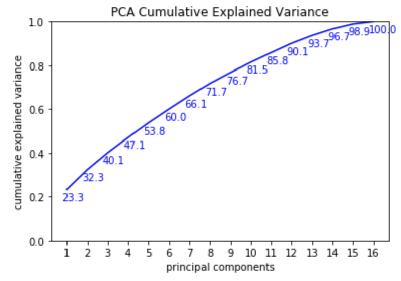
# Instantiate PCA with 10 principal components & fit to our dataset
pca = PCA(n_components=10, random_state=99).fit(X_scaled)

# Transform our dataset
X_scaled_red = pca.transform(X_scaled)
It’s important to understand that when dimensionality reduction is carried out using PCA, the outcome will be a set of new features which are linear combinations of the original features. Despite the loss of some interpretability that occurs when dimensionality reduction is performed using PCA, the benefits of utilizing lower dimensional data in the K-means clustering algorithm remain.
Implementing K-Means Clustering in Python
Building on the earlier introduction to K-means clustering and its methodology, it’s now time to put this technique into action. The first critical decision to make is the number of clusters, represented by the K parameter in K-means. There are various approaches to determining the optimal value of K, including evaluating silhouette scores; utilizing the elbow method on inertia values; looking at gap statistics; and considering the practicality of the number of clusters for your use case, such as whether 20 customer segments would be manageable for your marketing team.
# Instantiate KMeans class
clusterer = KMeans(n_clusters=6, random_state=99)

# Compute cluster centers and predict cluster for each sample
cluster_labels = clusterer.fit_predict(X_scaled_red)
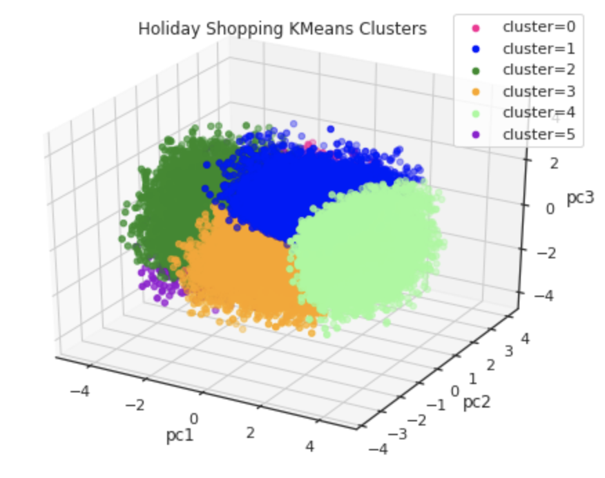
For this tutorial, we will set the number of clusters to six. The next step is to initialize the KMeans class and use the fit_predict method to apply the algorithm to our data. This will then assign each sample to one of the six clusters.
Next steps
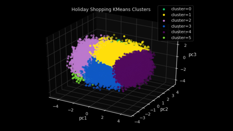
Next, we will evaluate the results and gain insights into the clustering by visualizing the clusters. Visualization tools such as pairplots and kernel density estimate plots are great for initial analysis. A 3D plot using Matplotlib can also provide a dynamic and interactive visualization of the cluster distributions, although it will only display three of the ten dimensions.
First, we will join the data that we input into the K-means algorithm with the cluster labels:
# Create DataFrame with samples and corresponding cluster labels
cluster_df = pd.DataFrame(data=X_scaled_red,
columns=['pc1','pc2','pc3','pc4','pc5','pc6','pc7','pc8','pc9','pc10'])
cluster_df['cluster'] = cluster_labels
Next, we will use Matplotlib’s mplot3d toolkit to create a 3D plot of our clusters.
# Define which features to plot
feature1 = 'pc1'
feature2 = 'pc2'
feature3 = 'pc3'

# Set up figure
fig = plt.figure(figsize=(8,6))
ax = plt.axes(projection='3d')

# Define our custom color list
color_list = ['deeppink', 'blue', 'forestgreen', 'orange', 'palegreen', 'darkviolet', 'moccasin', 'crimson', 'lightsteelblue', 'cyan']

# Iterate over each cluster, plotting on our figure
for i in range(cluster_df.cluster.nunique()):
label = "cluster=" + str(i)
  	ax.scatter3D(cluster_df[cluster_df.cluster==i][feature1],
	cluster_df[cluster_df.cluster==i][feature2],
     	cluster_df[cluster_df.cluster==i][feature3],
	c=color_list[i], label=label)

# Set labels and legend
ax.set_xlabel(feature1)
ax.set_ylabel(feature2)
ax.set_zlabel(feature3)
ax.set_title('Holiday Shopping KMeans Clusters')
ax.legend()
With the clusters identified, we could also join the cluster labels back to the original dataset to gain deeper insights into the consumer profile of each segment. This information can be used to develop descriptive segment names and profiles, which can help marketers better understand and communicate with their target audience. Additionally, the insights gained from this analysis can be used to inform marketing strategies and activate targeted campaigns. Please join me for my talk on May 9 at ODSC East 2023, where we will dive even deeper into the insights and applications of K-means clustering in marketing!