
Spatial Join
Spatial join combines attributes from one dataset to another based on their spatial relationship. To perform spatial join, specify geometry columns in both datasets and select the type of spatial join you want to perform. Once the operation is complete, you will receive a new joined dataset.
Perform a Spatial Join
On a dataset with a geometry column, click ⋮ More Options >> Spatial Join to open the spatial join configuration panel.
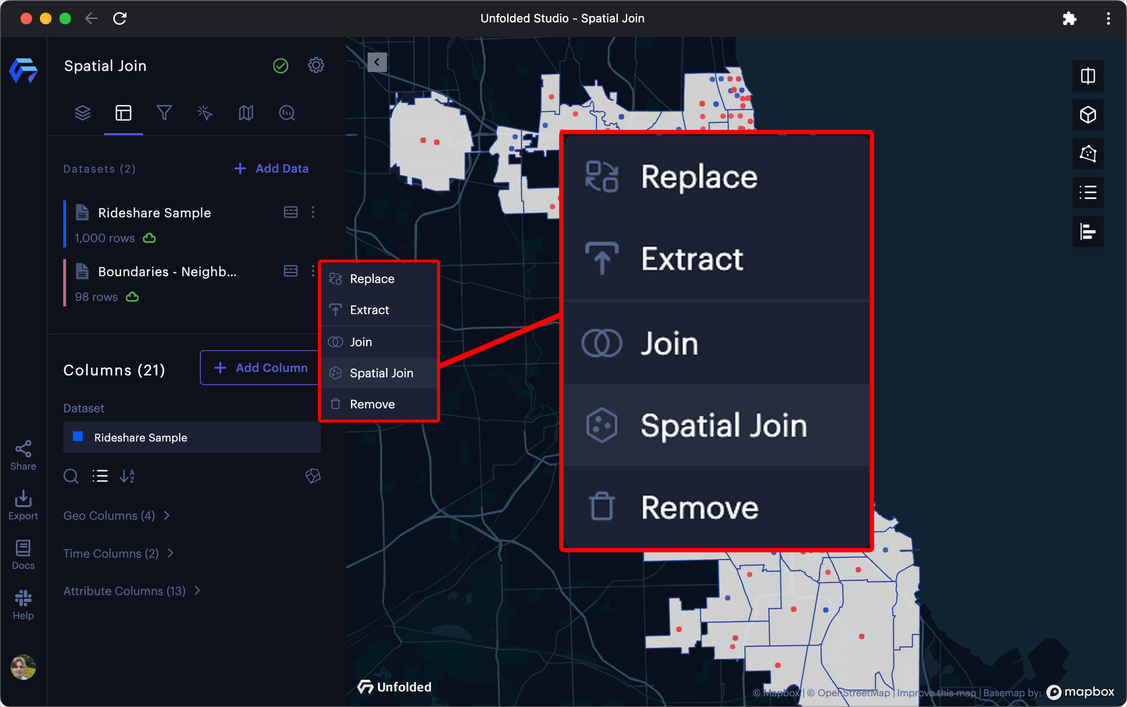
The Spatial Join button.
Spatial Join Configuration
The Spatial Join panel contains three sections:
- Target Dataset - configure the dataset you will join against.
- Join Operation - select a supported join operation between the source and target dataset.
- Join Dataset - select columns and specify aggregation rules (how to aggregate results when joining multiple rows). The supported aggregation rules include: Count, Sum, Mean, Max, Min, Deviation, Variance, Median, Percentile(P05, P25, P50, P75, P90)
Target Dataset
In the Target Dataset section, select a dataset containing a geometry column, select the geometry column, then select/deselect columns to include in the join operation.
Join Dataset
In the Join Dataset section, select a dataset to join, select a geometry column in that dataset, then specify aggregation rules.
Join Operation
Supported spatial join operations in Foursquare Studio:
| Join Operation | Description |
|---|---|
| Intersects | True when geometries share any portion of space. |
| Touches | True when geometries have at least one point in common, but their interiors do not intersect. |
| Within | True when geometry A is completely inside geometry B. |
| Overlaps | True when geometries share space but are not completely contained by each other. |
| Equals | True when geometries represent the same geometry. |
| Cross | True when geometries have some, but not all, interior points in common. |
Based on the geometry types you selected in both datasets, Foursquare Studio suggests an appropriate join type. However, you may select any combination of supported operations on the geometries of the datasets provided.
Click the Join Type dropdown to select a Join Type:
| Target | Join with | ||||||
|---|---|---|---|---|---|---|---|
| Intersects | Touches | Within | Overlaps | Equals | Crosses | ||
| Point | Point | ✔️ | ✔️ | ✔️ | |||
| MultiPoint | ✔️ | ✔️ | |||||
| Line/MultiLine | ✔️ | ✔️ | ✔️ | ||||
| Polygon/MultiPolygon | ✔️ | ✔️ | ✔️ | ||||
| MultiPoint | Point | ✔️ | ✔️ | ||||
| MultiPoint | ✔️ | ✔️ | ✔️ | ✔️ | |||
| Line/MultiLine | ✔️ | ✔️ | ✔️ | ✔️ | |||
| Polygon/MultiPolygon | ✔️ | ✔️ | ✔️ | ✔️ | |||
| Line/MultiLine | Point | ✔️ | ✔️ | ||||
| MultiPoint | ✔️ | ✔️ | ✔️ | ||||
| Line/MultiLine | ✔️ | ✔️ | ✔️ | ✔️ | ✔️ | ✔️ | |
| Polygon/MultiPolygon | ✔️ | ✔️ | ✔️ | ✔️ | |||
| Polygon/MultiPolygon | Point | ✔️ | ✔️ | ||||
| MultiPoint | ✔️ | ✔️ | ✔️ | ||||
| Line/MultiLine | ✔️ | ✔️ | ✔️ | ||||
| Polygon/MultiPolygon | ✔️ | ✔️ | ✔️ | ✔️ | ✔️ |
Aggregation Rules
When running any join operation, you must select an aggregation method for each selected column. Available methods depend on the data type of the column.

Aggregation options in Foursquare Studio.
The following aggregation methods are currently available in Studio:
| Aggregation Method | Column Type | Description |
|---|---|---|
| Count | string, datetime, number, | Counts the number of non-null values in the specified column. |
| Mode | string, datetime, number | Finds the most frequently occurring value(s) in the specified column. |
| Max | datetime, number | Returns the maximum value from the specified column. |
| Min | datetime, number | Returns the minimum value from the specified column. |
| Unique | string, number | Returns the count of distinct values in the specified column. |
| Sum | number | Computes the sum of all numeric values in the specified column. |
| Mean | number | Calculates the average (mean) value of all numeric values in the specified column. |
| Median | number | Returns the middle value in a sorted list of numeric values in the specified column. |
| Variance | number | Measures the variability (spread) of numeric values in the specified column from their mean. |
| Deviation | number | Calculates the standard deviation of numeric values in the specified column. |
| P05 | number | Returns the value below which 5% of the data falls in the specified column. |
| P25 | number | Returns the value below which 25% of the data falls in the specified column. |
| P50 | number | Returns the value below which 50% of the data falls (same as the median) in the column. |
| P75 | number | Returns the value below which 75% of the data falls (same as the median) in the column. |
| P95 | number | Returns the value below which 95% of the data falls in the specified column. |
Spatial Join Examples
Spatial join is one of the most popular geoprocessing tools in GIS. Here are some examples of practical uses of applying a spatial join using Foursquare Studio:
Example 1. Aggregate the parking infractions data for 157 neighborhoods in Philadelphia.
The parking infractions data include millions of points that each one represents the location of a parking violation ticket. Using spatial join, we can aggregate the points to each neighborhood based on the geographic locations.
In this example, we demonstrate how to compute the total dollar amount fined via parking violations for all neighborhoods in Philadelphia:
-
Select the
Spatial Joinoption from the dataset "Neighborhoods_Philadelphia.json". -
In the Spatial Join panel, select the
Join Dataset: "Parking Violations.csv". Foursquare Studio will automatically detect the geometry type "Point" and geometry column: "lat" and "lon". -
Ensure the
Join Operationselection isIntersects, which means all the points within or touch the polygon are considered as valid spatial join. -
Click on the field selector of
finecolumn under theAttribute Columns(1)label, and chooseSumas the aggregation rule in the pop-up menu. By doing so, we can compute the sum of thefinevalue of all points joined with each neighborhood.
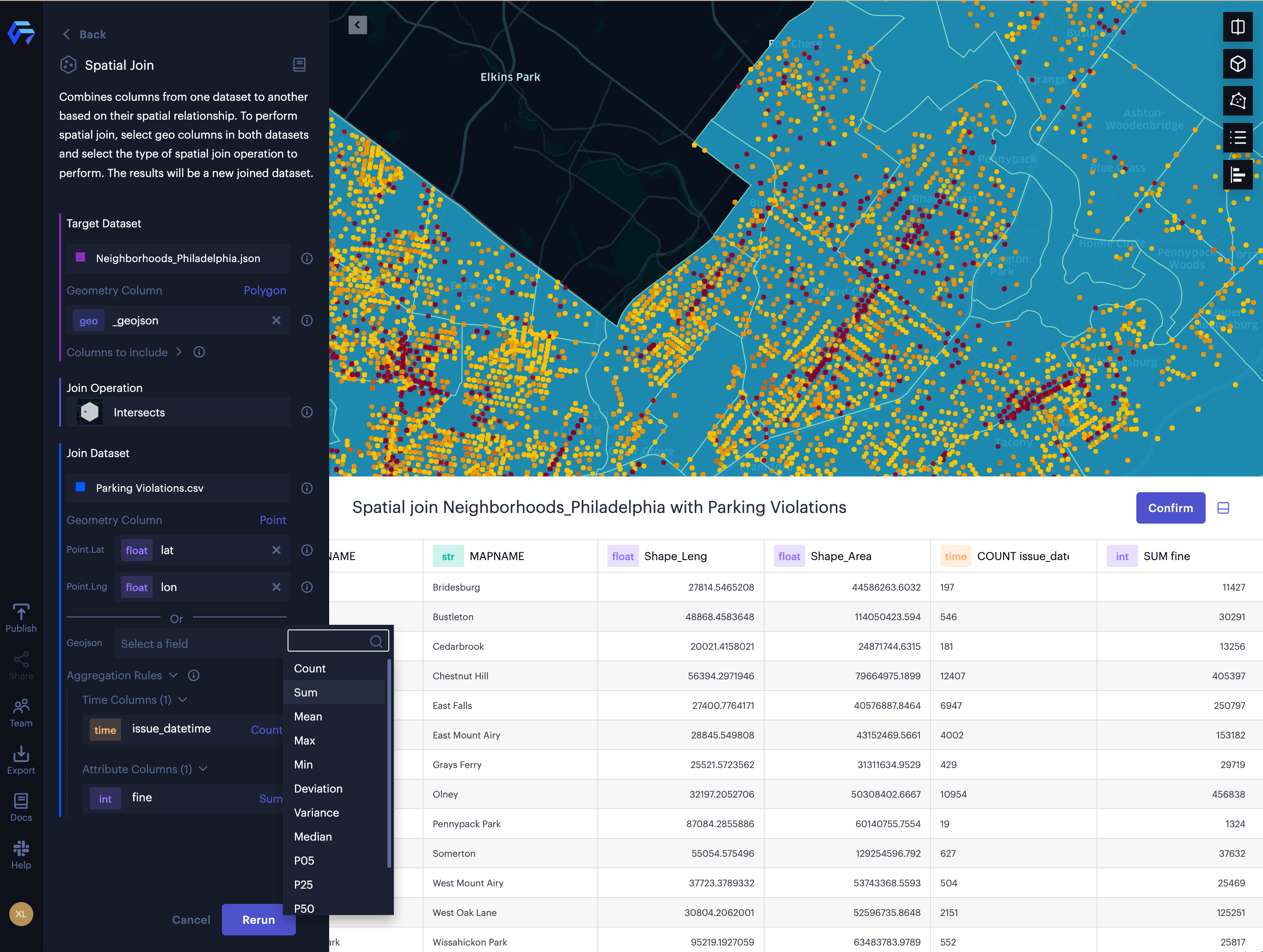
Spatial join the parking infractions data with 157 neighborhoods in Philadelphia.
The result of the spatial join is a new dataset with a column COUNT issue_date, which represents how many data points (tickets) are in each polygon (neighborhood), and a column SUM fine, which represents the total amount of fine from all data points in each neighborhood. Then, we can create a thematic map using the new column SUM fine to show the spatial distribution of the infractions data at the neighborhood level (see Figure 3).
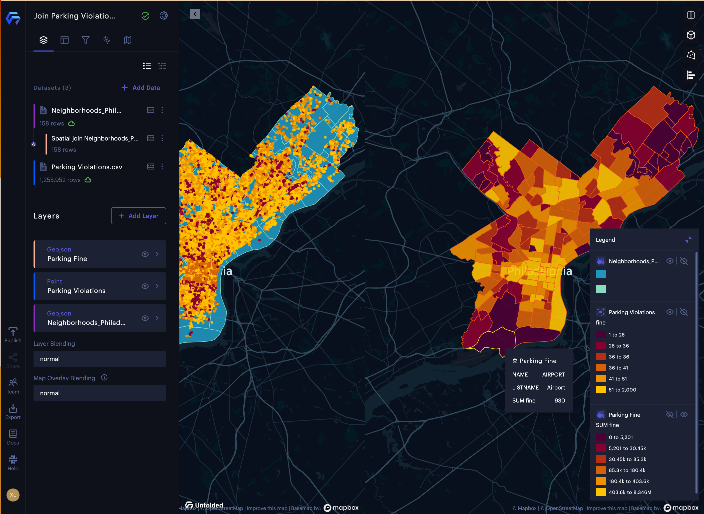
The result of spatial join the parking infractions data with 157 neighborhoods in Philadelphia.
Example 2. Spatial join the building footprints with 25 Zip code areas in San Francisco.
In this example, we are going to spatial joining 25 zip code areas with 177,023 building footprints in San Francisco, so we can compute how many buildings and the total area they occupy in each zip code area.
- Select the
Spatial Joinoption from the dataset "sfzip.json". - In the Spatial Join panel, we select the
Join Dataset: "sf.buildings.json". Studio studio will automatically detect the geometry type "Polygon" and geometry column: "_geojson". - Ensure the
Join OperationisIntersects, which means all the polygons (buildings) intersect with the zip code area are considered as valid spatial join. - Click on the field selector of
mblr(San Francisco property key) column under theAttribute Columns(2)label, and chooseCountas the aggregation rule in the pop-up menu. By doing so, we can count how many building footprints intersect with each zip code area. - Click on the field selector of
area(The area of building in square meters) column under theAttribute Columns(2)label, and chooseSumas the aggregation rule in the pop-up menu. By doing so, we can compute the total area of the building footprints intersect with each zip code area.
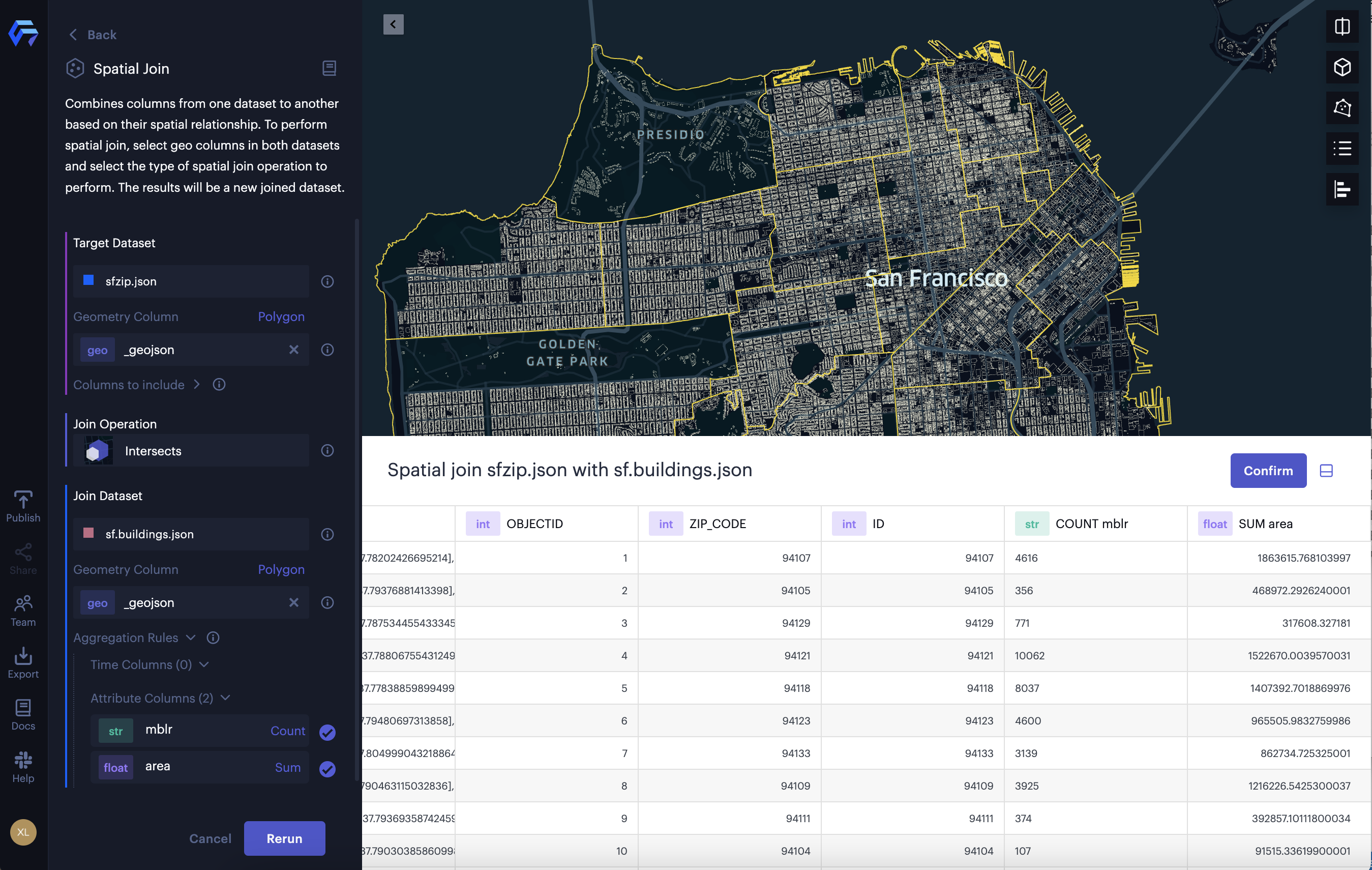
Spatial join the building footprints with zip code area in San Francisco.
The result of the spatial join is a new dataset with a column COUNT mlbr, which represents how many building footprints in each zip code area, and a column SUM area, which represents the total area of the building footprints in each zip code area. Then, we can create a thematic map using the new column SUM area to show the spatial distribution of the total area of building footprints at the zip code level (see Figure 5).
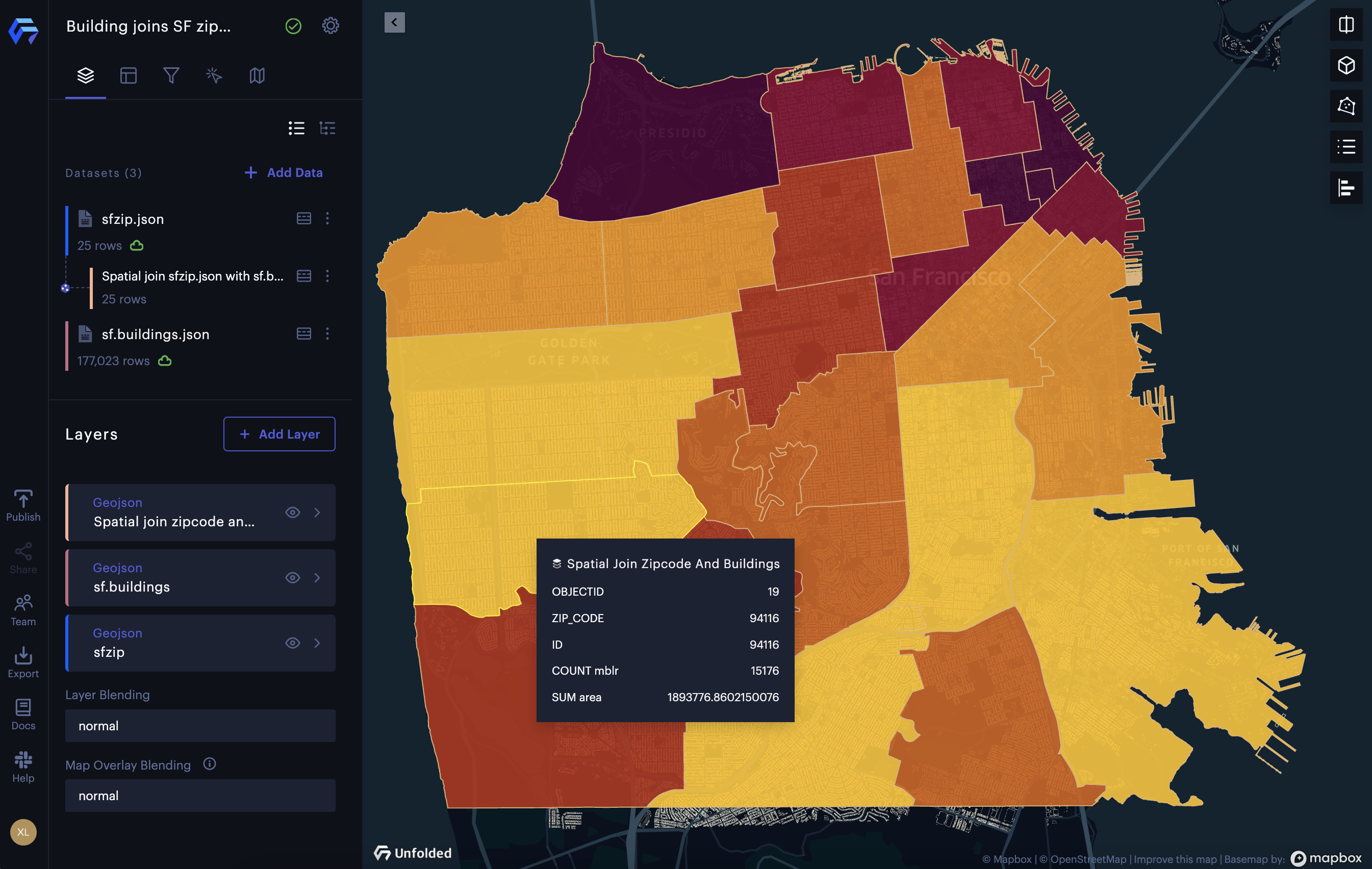
The result of spatial join the building footprints with zip code area in San Francisco.
Updated 3 months ago