
Origin-Destination Analysis
Origin-Destination data represents numbers of movements between pairs of geographic locations. OD-data analysis can help with finding patterns in e.g. traffic flows, commutes, migrations, and other transportation.
Every origin-destination data record includes a pair of locations:
- An Origin (or Source) location.
- A Destination (or Target) location.
Data representing movement such as trips, deliveries, and foot traffic naturally contain these locations, making them well suited for an origin-destination analysis.
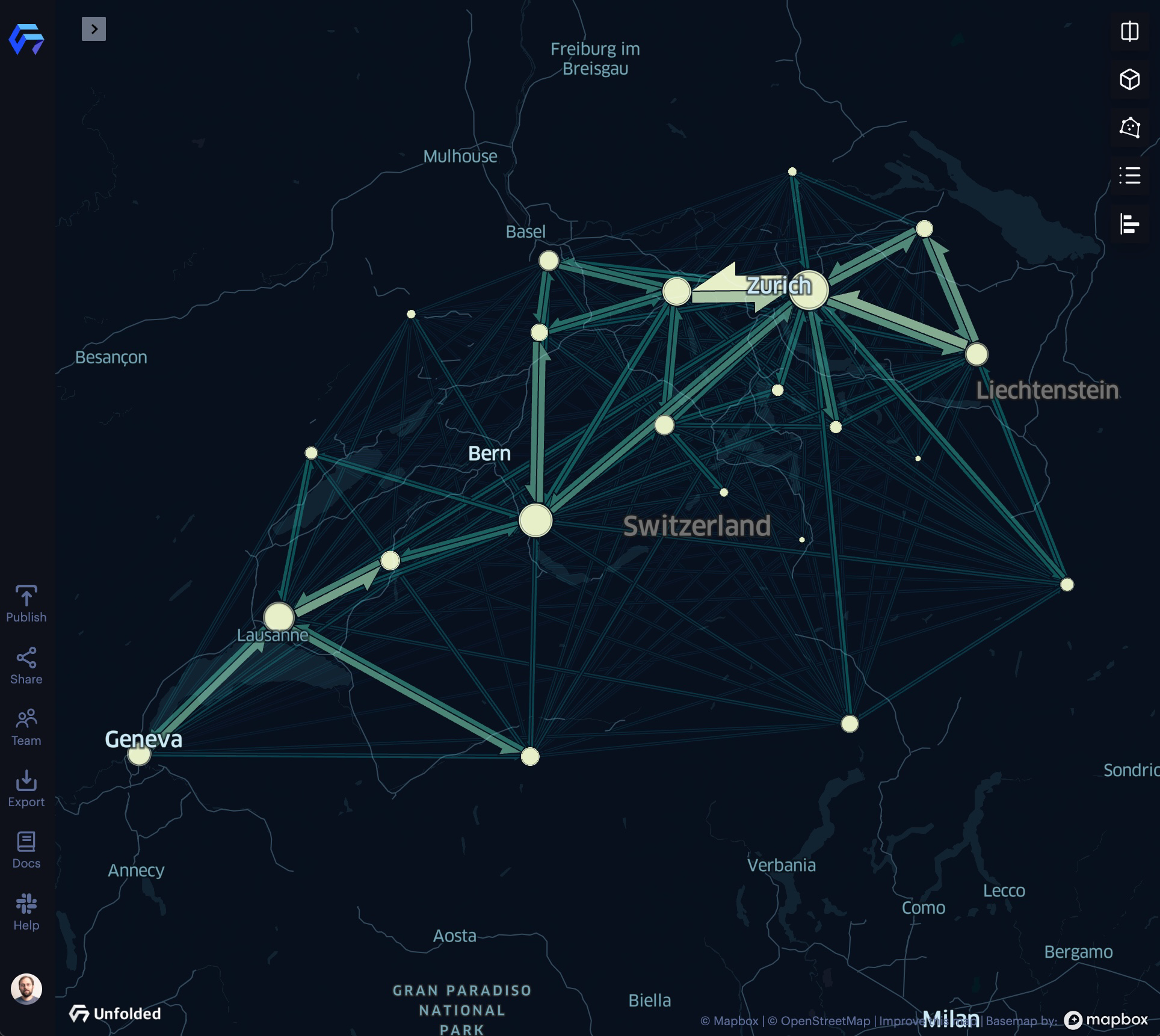
An example of origin-destination visualization with the Flow Layer.
Tip: If your dataset is more granular, containing detailed paths with additional data such as timestamps, you can use Fleet Visualization techniques to create powerful visualizations.
Line Layer
Show line connections between origins and destinations with the Line Layer.
The Line Layer is best in datasets with few points, as datasets with too many points show many intersecting lines, making it hard to discern patterns in the visualization.
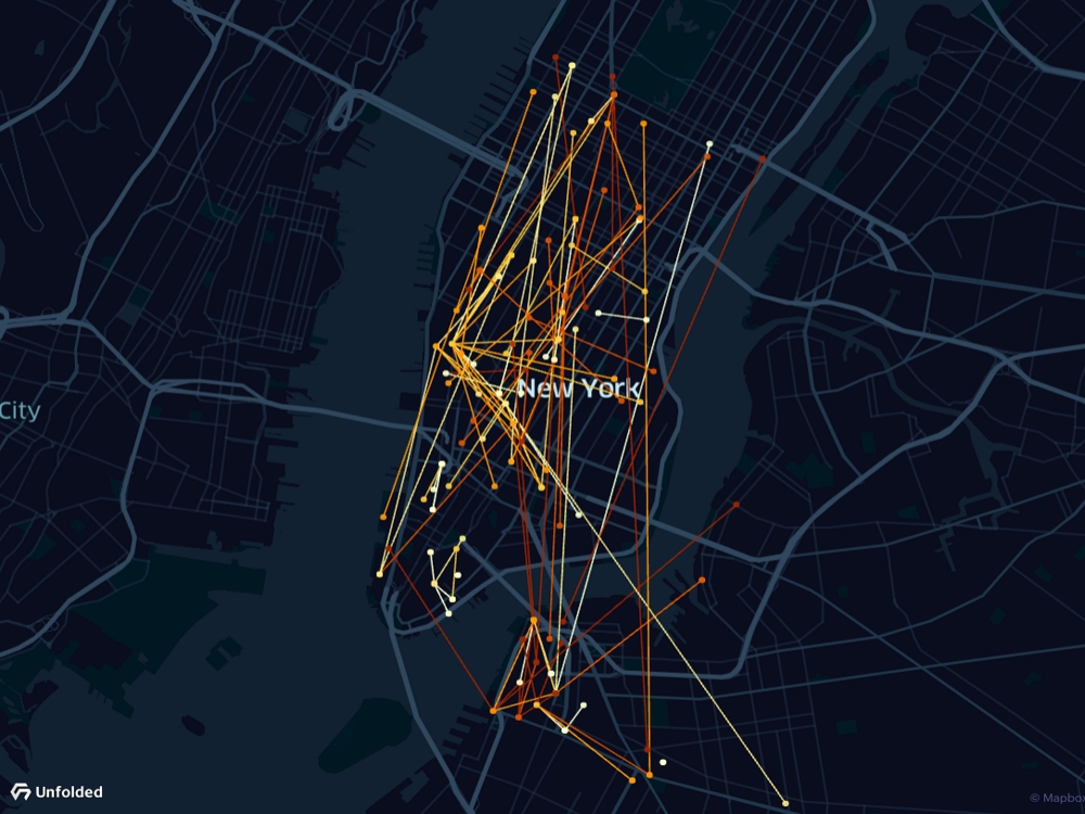
The Line Layer.
Arc Layer
Show arcs between origins and destinations with the Arc Layer.
Arcs use the third dimension to detangle intersecting lines, providing increased clarity in larger datasets.
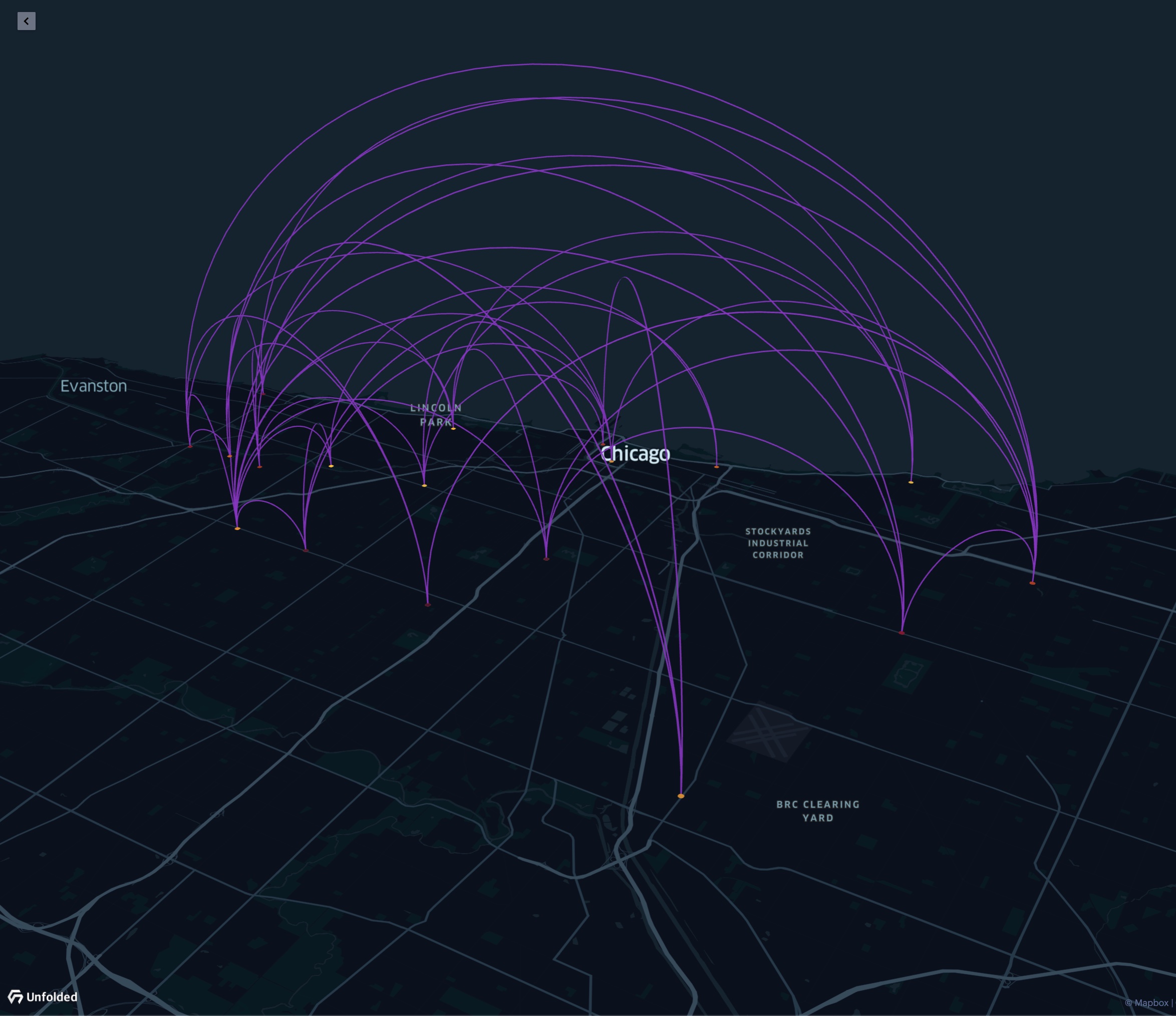
The Arc Layer.
Color by Origin and Destination
Arc Layers can be configured to emphasize trends in your origin-destination analysis. For example, you can use colors to identify origins and destinations in the Arc Layer. This better shows the direction of movement and helps visually distinguish more arcs.
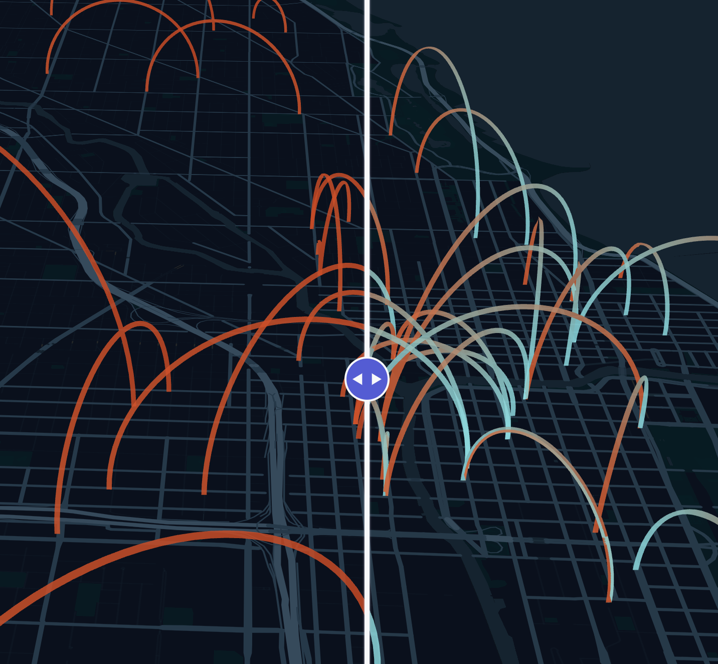
Left: A solid-colored Arc Layer. Right: An Arc Layer colored by origin (blue) and destination (red).
Blending
While the Arc Layer uses the third dimension to detangle lines, crowding and overlapping may occur in large datasets. In visualizations with a large number of overlapping arcs, you can enable Additive Blending Mode.
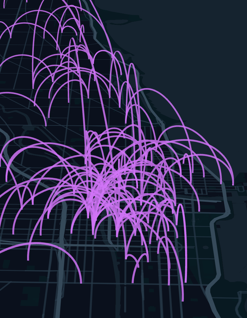 | 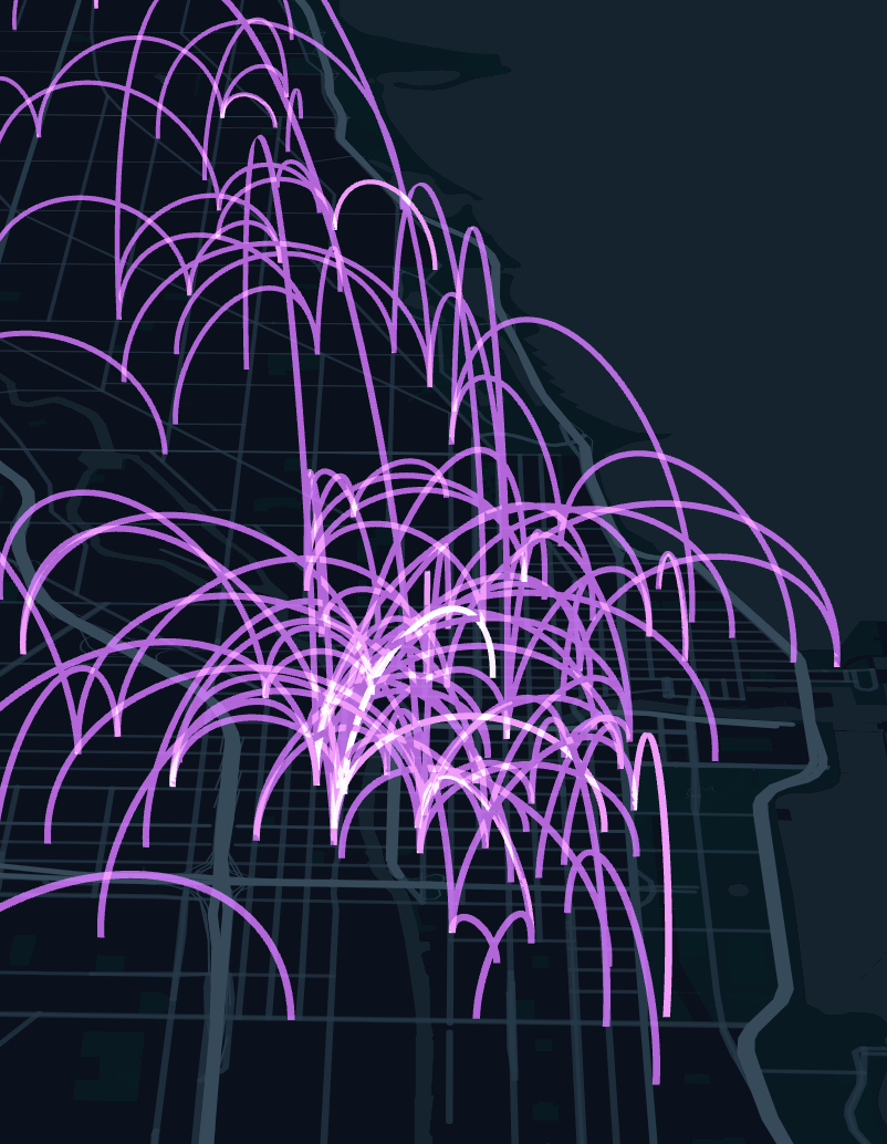 |
|---|---|
The above Arc Layer example experiences overlapping in the city center. Notice that when Additive Blending is enabled, overlapping arcs are exposed via increased brightening intensity.
Brushing
Brushing allows you to visually explore large datasets by restricting the visualization to areas surrounding the cursor, allowing you to focus on trends in a specific area.
The Brush tool works particularly well with Arc Layers, allowing users to focus on localized trends in crowded datasets.
Brushing on a busy Arc Layer.
Arc Layer Example Map
Flow Layer
While the Arc Layer in combination with blending and brushing makes it possible to visualize and explore origin-destination data, you may need to explore your data with an aggregated view.
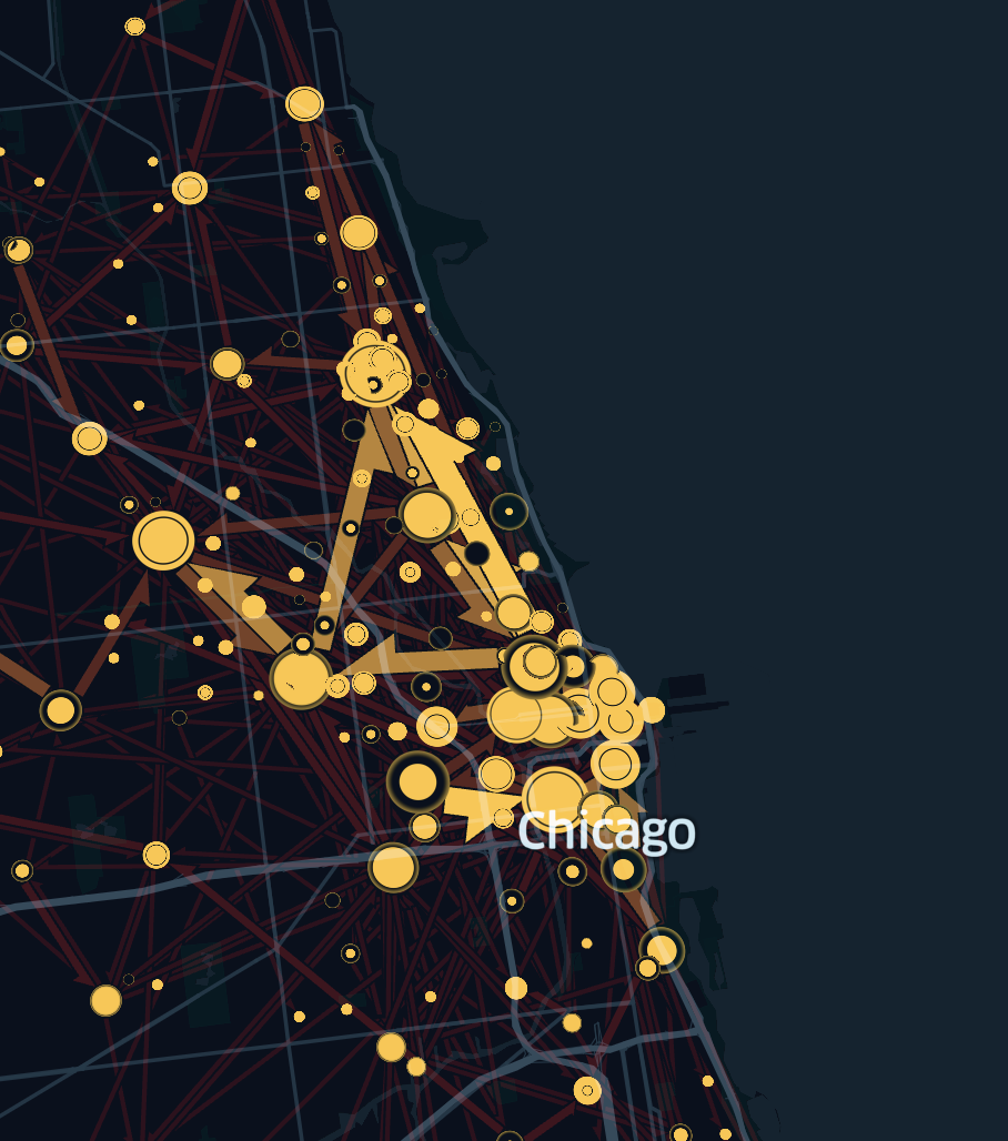
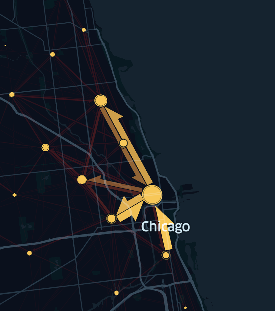
The Flow Layer is an effective way of visualizing aggregated origin-destination movement patterns.
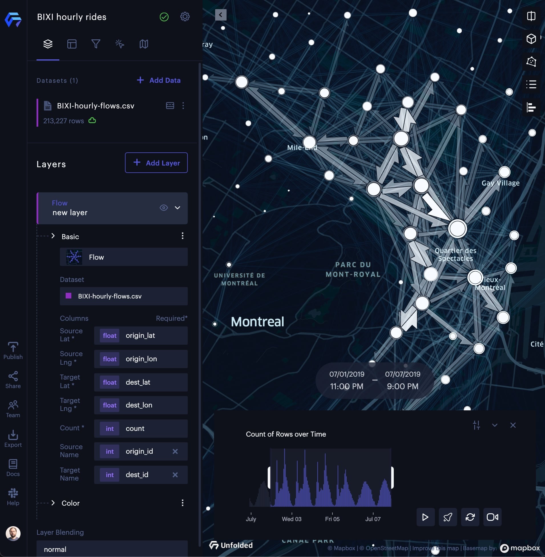
The Flow Layer.
Emphasize Flows with Higher Traffic
To highlight key traffic patterns, the Fade slider enables you to de-emphasize flows with less traffic.
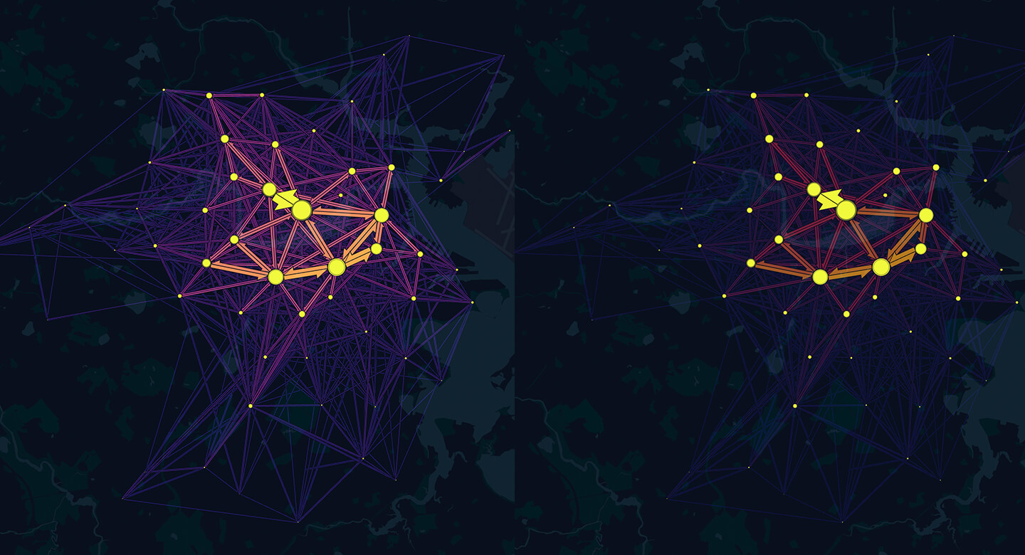
Left: Fade = 0; Right: Fade = 30.
Show Traffic Totals per Location
In addition to emphasizing the flows between locations, it is also possible to highlight the amount of traffic flowing to and from each location.
The Location Totals toggle makes the size of the location total circles is based on the number of flows in and out of the location.
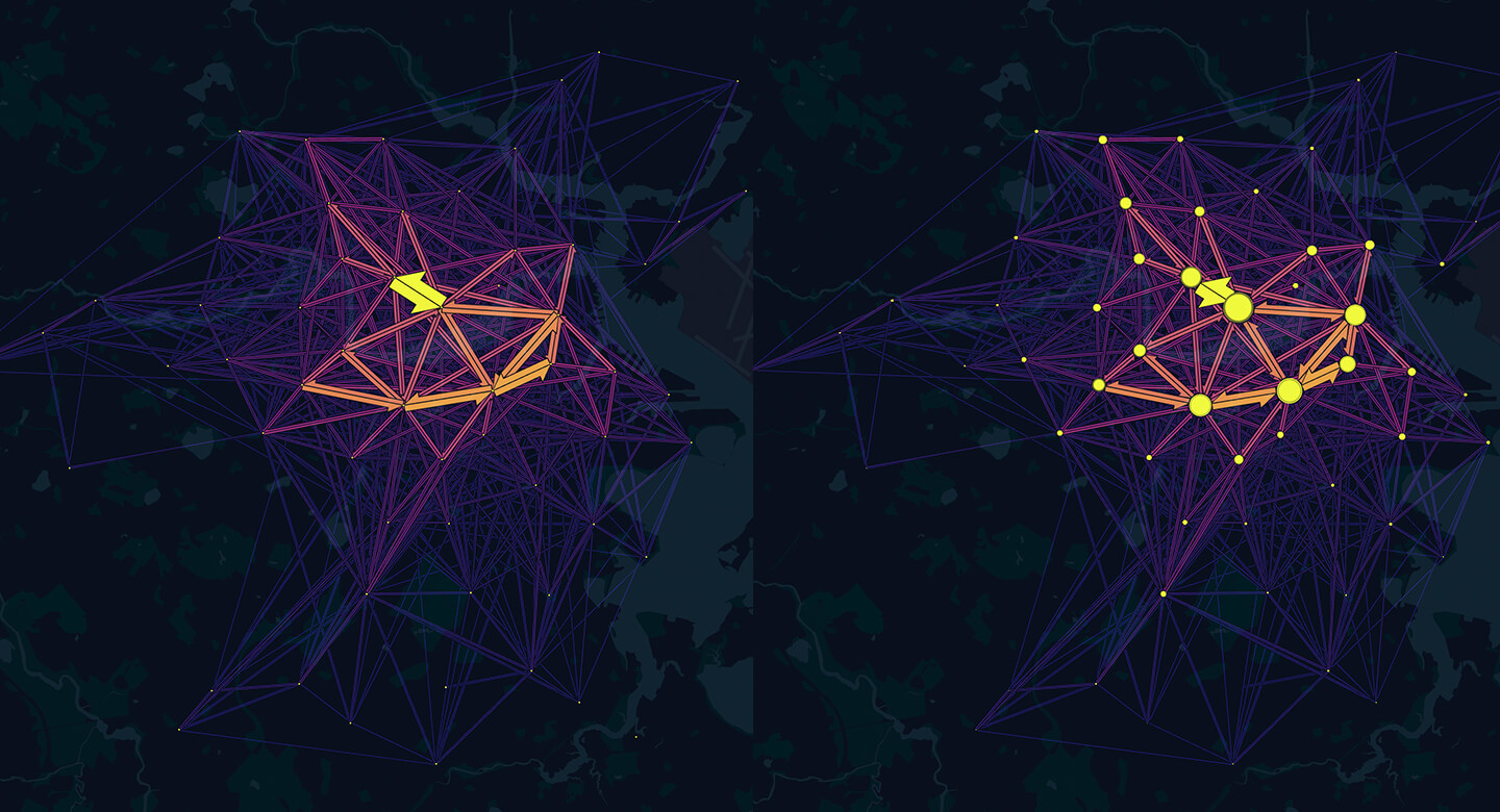
Left: Location totals off; Right: Location totals on.
Animate Flows
To highlight movement, animate your flows via the Animation toggle.
By animating flows, movement such as taxi, bike, and rideshare trips feels more active and kinetic.
Flow Layer animation.
Cluster Origin and Destination Points
The Flow Layer can automatically group origins and destinations with hierarchical agglomerative clustering using screen pixel distance as the distance metric.
Use the Clustering toggle to enable/disable clustering of flow origins and destinations. Clustering groups nearby source-target points and increases visibility while adapting as you zoom in and out.
 |  |
|---|
To Cluster or Not to Cluster
In flow mapping, flow patterns are discovered based on predefined clusters or arbitrary clusters detected by clustering algorithms. However, different clustering algorithms can generate different arbitrary clusters, leading to different flow patterns. This phenomenon is referred to as the Modifiable Areal Unit Problem (MAUP).
For pre-determined analytical units like bike-sharing stations, the MAUP effect could be ignored in flow mapping. Therefore, it is often preferable to not cluster when the dataset has a natural structure, such as datasets containing fixed pick-up and drop-off locations for rental fleets of cars and scooters, which usually start and end in well-defined places.
However, when you need to extract structure (e.g. arbitrary clusters) from large datasets with "random" origins and destinations, such as datasets containing random pick-up and drop-off locations for taxi or rideshare scenarios, it is preferable to enable clustering to discover flow patterns based on these arbitrary clusters. To help analysts deal with the MAUP effect, the flow layer in Foursquare Studio offers a hierarchical agglomerative clustering approach using screen pixel distance as the proximity measure. It provides an interactive experience enabling analysts to explore and evaluate flow patterns at different spatial scales.
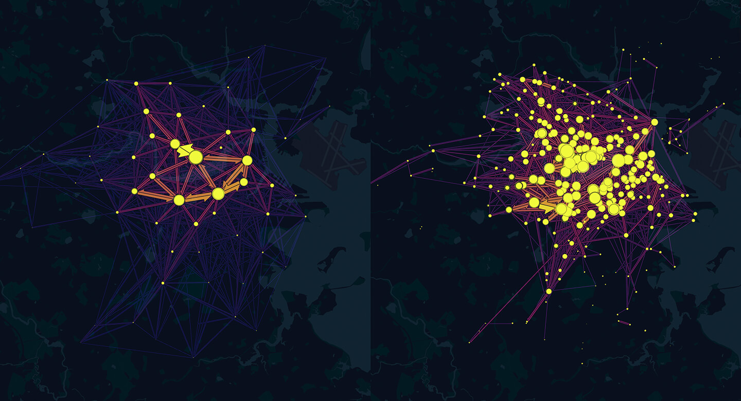
An animation showing how clusters and flows change as you zoom in and out.
When zoomed out, clusters are created at a large spatial scale (e.g. county or city level) and provide a better summary of the overall origin-destination network structure and the flow patterns. This summary view can help to reveal the big picture from the flow map. Dense areas with many short origin-destination flows, such as rideshare data within a city center, are not obscured as the user zooms out. Additionally, while zoomed in, clusters are created at a small spatial scale (e.g. zip-code or street level) with flow patterns that expose a finer level of detail. In the right scenarios, clustering helps analysts address the issue of MAUP in flow mapping, granting the ability to choose the right spatial scale for evaluation.
Cluster Layer Example Map
Updated 3 months ago